Minimizing Cost

비용 최소화 코드

저번글에서 X, Y에 최적화된 W, b를 찾았다면, 이번에는 고정된 X, Y 에 대해 다른 W값을 넣어주면서 Cost의 변화를 살펴보자.

# Lab 3 Minimizing Cost
import tensorflow as tf
import matplotlib.pyplot as plt
 
# 고정된 데이터 셋
X = [1, 2, 3]
Y = [1, 2, 3]
 
# W값을 변화시키며 관찰할 것이므로 placeholder로 선언해준다.
W = tf.placeholder(tf.float32)
 
# Our hypothesis for linear model X * W
# 간단한 1차함수로 선언해보자.
hypothesis = X * W
 
# cost/loss function
# 비용함수는 MSE로 한다.
cost = tf.reduce_mean(tf.square(hypothesis - Y))
 
# Variables for plotting cost function
# W값에 따른 Cost의 변화를 알아볼 것이므로 그래프를 실행하면서 값을 저장할 빈 list를 만들어준다.
W_history = []
cost_history = []
 
# Launch the graph in a session.
with tf.Session() as sess:
    for i in range(-30, 50):
        curr_W = i * 0.1
        curr_cost = sess.run(cost, feed_dict={W: curr_W})
 
        W_history.append(curr_W)
        cost_history.append(curr_cost)
 
# Show the cost function
plt.plot(W_history, cost_history)
plt.show()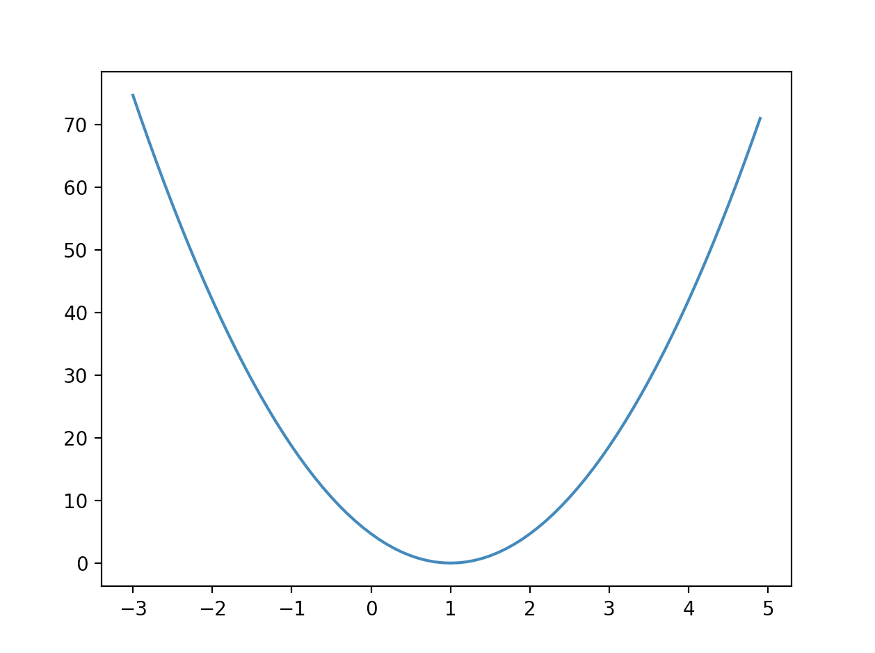

W = 1 일때, cost가 최소가 된다.

Gradient Descent

$$W=W-\alpha \frac{1}{m}\sum \_{i=1}^m(W{x}^{(i)}-y^{(i)})x^{(i)}$$

W를 다음과 같은 방식으로 업데이트하는 것이 W의 최소를 찾도록 한다.

아까 minimize 할 때 사용했던 코드를 우리가 다음의 코드로 바꿀 수 있다.

# Minimize: Gradient Descent using derivative: W -= learning_rate * derivative
learning_rate = 0.1
gradient = tf.reduce_mean((W * X - Y) * X)
descent = W - learning_rate * gradient
update = W.assign(descent)

그리고 나서 세션을 실행해줘야 하므로,

# Launch the graph in a session.
with tf.Session() as sess:
    # Initializes global variables in the graph.
    sess.run(tf.global_variables_initializer())
 
    for step in range(21):
        _, cost_val, W_val = sess.run(
            [update, cost, W], feed_dict={X: x_data, Y: y_data}
        )
        print(step, cost_val, W_val)
 
"""

0 6.8174477 [1.6446238]
1 1.9391857 [1.3437994]
2 0.5515905 [1.1833596]
3 0.15689684 [1.0977918]
4 0.044628453 [1.0521556]
5 0.012694317 [1.0278163]
6 0.003610816 [1.0148354]
7 0.0010270766 [1.0079122]
8 0.00029214387 [1.0042198]
9 8.309683e-05 [1.0022506]
10 2.363606e-05 [1.0012003]
11 6.723852e-06 [1.0006402]
12 1.912386e-06 [1.0003414]
13 5.439676e-07 [1.000182]
14 1.5459062e-07 [1.000097]
15 4.3941593e-08 [1.0000517]
16 1.2491266e-08 [1.0000275]
17 3.5321979e-09 [1.0000147]
18 9.998237e-10 [1.0000079]
19 2.8887825e-10 [1.0000042]
20 8.02487e-11 [1.0000023]

초기 Weight를 다르게 줘보자.

# Lab 3 Minimizing Cost
import tensorflow as tf
 
# tf Graph Input
X = [1, 2, 3]
Y = [1, 2, 3]
 
# Set wrong model weights
W = tf.Variable(5.0)
 
# Linear model
hypothesis = X * W
 
# cost/loss function
cost = tf.reduce_mean(tf.square(hypothesis - Y))
 
# Minimize: Gradient Descent Optimizer
train = tf.train.GradientDescentOptimizer(learning_rate=0.1).minimize(cost)
 
# Launch the graph in a session.
with tf.Session() as sess:
    # Initializes global variables in the graph.
    sess.run(tf.global_variables_initializer())
 
    for step in range(101):
        _, W_val = sess.run([train, W])
        print(step, W_val)
 

 
0 5.0
1 1.2666664
2 1.0177778
3 1.0011852
4 1.000079
...
97 1.0
98 1.0
99 1.0
100 1.0
 

Tensorflow에게 Gradient 구하게 해보기

위의 예제 에서 우리는

$$MSE=\frac{1}{m}\sum \_{i=1}^m(W{x}^{(i)}-y^{(i)}{)}^2$$

MSE 함수의 Gradient 를 구해, gradient라는 변수에 넣어주었다.

$$diff(MSE)=\frac{2}{m}\sum \_{i=1}^m(W{x}^{(i)}-y^{(i)})x^{(i)}$$

gradient = tf.reduce_mean((W * X - Y) * X)

그런데, MSE만 정의해주고, tensorflow한테 이걸 시킬 수 있다.

또한 미분까지만 정의하고, 그 값에서 내가 추가적인 행동 역시 할 수 있다.

# Lab 3 Minimizing Cost
# This is optional
import tensorflow as tf
 
# tf Graph Input
X = [1, 2, 3]
Y = [1, 2, 3]
 
# Set wrong model weights
W = tf.Variable(5.)
 
# Linear model
hypothesis = X * W
 
# Manual gradient
# 위에서는 2가 없지만, 
gradient = tf.reduce_mean((W * X - Y) * X) * 2
 
# cost/loss function
cost = tf.reduce_mean(tf.square(hypothesis - Y))
 
# Gradient Descent Optimizer
optimizer = tf.train.GradientDescentOptimizer(learning_rate=0.01)
 
# optimize 까지 선언하고 .minizize(cost)를 쓰게 되면, 기본적인
# Gradient descent가 진행된다.
# 그런데 이함수를 쓰지말고, 여기서 .compute_gradients(cost)를 쓰게되면,
# 이 cost 함수에 대한 gradient를 계산해준다.
# 즉 미분한 값을 돌려준다.
# Get gradients
gvs = optimizer.compute_gradients(cost)
 
# 여기서 모델을 수정하기 위해 다른 작업이 필요하면 하면된다.
# Optional: modify gradient if necessary
# gvs = [(tf.clip_by_value(grad, -1., 1.), var) for grad, var in gvs]
 
# Apply gradients
# 이 변화한 gvs 값을 다시 optimizer에 돌려줄 수 있다.
apply_gradients = optimizer.apply_gradients(gvs)
 
# Launch the graph in a session.
with tf.Session() as sess:
    # Initializes global variables in the graph.
    sess.run(tf.global_variables_initializer())
 
    for step in range(101):
        gradient_val, gvs_val, _ = sess.run([gradient, gvs, apply_gradients])
        print(step, gradient_val, gvs_val)
 
'''
0 37.333332 [(37.333336, 5.0)]
1 33.84889 [(33.84889, 4.6266665)]
2 30.689657 [(30.689657, 4.2881775)]
3 27.825289 [(27.825289, 3.981281)]
...
97 0.0027837753 [(0.0027837753, 1.0002983)]
98 0.0025234222 [(0.0025234222, 1.0002704)]
99 0.0022875469 [(0.0022875469, 1.0002451)]
100 0.0020739238 [(0.0020739238, 1.0002222)]
'''