Linear Regression

Code

import tensorflow as tf
tf.set_random_seed(777)  # 같은 값이 나오도록 하기 위해서
 
# 데이터 준비
x_train = [1, 2, 3]
y_train = [1, 2, 3]
 
# 초기에 랜덤하게 값을 할당한다.
W = tf.Variable(tf.random_normal([1]), name = 'weight')
b = tf.Variable(tf.random_normal([1]), name="bias")
 
# 우리의 가설, XW + b
# 선형으로 생겼을 것이다, 예측값
hypothesis = x_train * W + b

Cost function으로 MSE를 사용할 것이므로,

# cost/loss function
cost = tf.reduce_mean(tf.square(hypothesis - y_train))

이제, 데이터가 주어졌고, 어떤 Cost function을 최적화할지도 정해졌으니,

어떤 알고리즘으로 최적화할지 결정해야 한다.

기본적으로 우리는 Gradient Descent를 사용하도록 하겠다.

# optimizer
optimizer = tf.train.GradientDescentOptimizer(learning_rate = 0.01)
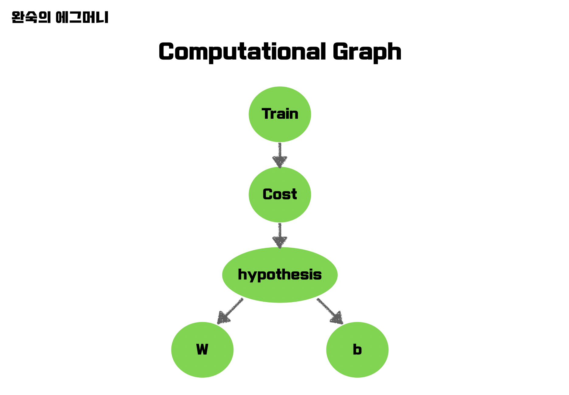
train = optimizer.minimize(cost)

여기까지 Tensorflow를 사용함에 있어서 Computation Graph를 다 그렸다고 생각하면 된다.

이제 실행해야 하므로, session을 수행하자.

sess = tf.Session()

그런데 우리가 변수로 지정해 놓은 W, b를 사용하기 전에는 항상 초기화 를 해주어야 한다.

sess.run(tf.global_variables_initializer())

이제 실행시킬 준비가 되었고, 우리는 총 2000번 training을 수행하고 싶다.

이때 실행시키고 싶은 노드는 train 이다.

for step in range(2001):
    sess.run(train)

그런데 이럴 경우 어떻게 잘 fitting이 되었는지 알 수 없으므로, 다른 값을을 print해보자.

우리가 조사하고 싶은 값은,

1. step에 따라서
2. cost가 어떻게 변화했는지
3. W가 어떻게 변화했는지
4. b가 어떻게 변화했는지 이다.

for step in range(2001):
    sess.run(train)
    if step % 20 == 0:
        print(step, sess,run(cost), sess.run(W), sess.run(b))

먼저 2001번 반복을 진행하고,

2000번 print를 하지말고 200번만 하도록 하자.

노드를 실행시켜야 그 결과값을 알 수 있으므로 내가 조사하고 싶은 노드를 모두 session으로 실행시키고

그 결과값을 print하자.

전체코드

import tensorflow as tf
tf.set_random_seed(777)  # 같은 값이 나오도록 하기 위해서
 
# 데이터 준비
x_train = [1, 2, 3]
y_train = [1, 2, 3]
 
# 초기에 랜덤하게 값을 할당한다.
W = tf.Variable(tf.random_normal([1]), name = 'weight')
b = tf.Variable(tf.random_normal([1]), name="bias")
 
# 우리의 가설, XW + b
# 선형으로 생겼을 것이다, 예측값
hypothesis = x_train * W + b
 
# cost/loss function
cost = tf.reduce_mean(tf.square(hypothesis - y_train))
 
# optimizer
optimizer = tf.train.GradientDescentOptimizer(learning_rate = 0.01)
train = optimizer.minimize(cost)
 
# session 노드 만들기
sess = tf.Session()
 
# 변수 초기화하기
sess.run(tf.global_variables_initializer())
 
# 훈련 진행, printing
for step in range(2001):
    sess.run(train)
    if step % 20 == 0:
        print(step, sess,run(cost), sess.run(W), sess.run(b))

이 때, with 문을 사용하여 조금더 간결하게 사용할 수 있다.

또한, 내가 필요한 노드들을 변수로 처음부터 받은 뒤,

출력해주는게 보다 깔끔하다.

# Launch the graph in a session.
with tf.Session() as sess:
    # Initializes global variables in the graph.
    sess.run(tf.global_variables_initializer())
 
    # Fit the line
    for step in range(2001):
        _, cost_val, W_val, b_val = sess.run([train, cost, W, b])
 
        if step % 20 == 0:
            print(step, cost_val, W_val, b_val)

• 결과

  0 3.5240757 [2.1286771] [-0.8523567]
  20 0.19749945 [1.533928] [-1.0505961]
  40 0.15214379 [1.4572546] [-1.0239124]
  60 0.1379325 [1.4308538] [-0.9779527]
  80 0.12527025 [1.4101374] [-0.93219817]
  100 0.11377233 [1.3908179] [-0.8884077]
  120 0.10332986 [1.3724468] [-0.8466577]
  140 0.093845844 [1.3549428] [-0.80686814]
  160 0.08523229 [1.3382617] [-0.7689483]
  180 0.07740932 [1.3223647] [-0.73281056]
  200 0.07030439 [1.3072149] [-0.6983712]
  220 0.06385162 [1.2927768] [-0.6655505]
  240 0.05799109 [1.2790174] [-0.63427216]
  260 0.05266844 [1.2659047] [-0.6044637]
  280 0.047834318 [1.2534081] [-0.57605624]
  300 0.043443877 [1.2414987] [-0.5489836]
  320 0.0394564 [1.2301493] [-0.5231833]
  340 0.035834935 [1.2193329] [-0.49859545]
  360 0.032545824 [1.2090251] [-0.47516325]
  380 0.029558638 [1.1992016] [-0.45283225]
  400 0.026845641 [1.18984] [-0.4315508]
  420 0.024381675 [1.1809182] [-0.41126958]
  440 0.02214382 [1.1724157] [-0.39194146]
  460 0.020111356 [1.1643128] [-0.37352163]
  480 0.018265454 [1.1565907] [-0.35596743]
  500 0.016588978 [1.1492316] [-0.33923826]
  520 0.015066384 [1.1422179] [-0.3232953]
  540 0.01368351 [1.1355343] [-0.30810148]
  560 0.012427575 [1.1291647] [-0.29362184]
  580 0.011286932 [1.1230947] [-0.2798227]
  600 0.010250964 [1.1173096] [-0.26667204]
  620 0.009310094 [1.1117964] [-0.25413945]
  640 0.008455581 [1.1065423] [-0.24219586]
  660 0.0076795053 [1.1015354] [-0.23081362]
  680 0.006974643 [1.0967635] [-0.21996623]
  700 0.0063344706 [1.0922159] [-0.20962858]
  720 0.0057530706 [1.0878822] [-0.19977672]
  740 0.0052250377 [1.0837522] [-0.19038804]
  760 0.004745458 [1.0798159] [-0.18144041]
  780 0.004309906 [1.076065] [-0.17291337]
  800 0.003914324 [1.0724902] [-0.16478711]
  820 0.0035550483 [1.0690835] [-0.1570428]
  840 0.0032287557 [1.0658368] [-0.14966238]
  860 0.0029324207 [1.0627428] [-0.14262886]
  880 0.0026632652 [1.059794] [-0.13592596]
  900 0.0024188235 [1.056984] [-0.12953788]
  920 0.0021968128 [1.0543059] [-0.12345006]
  940 0.001995178 [1.0517538] [-0.11764836]
  960 0.0018120449 [1.0493214] [-0.11211928]
  980 0.0016457299 [1.0470035] [-0.10685005]
  1000 0.0014946823 [1.0447946] [-0.10182849]
  1020 0.0013574976 [1.0426894] [-0.09704296]
  1040 0.001232898 [1.0406833] [-0.09248237]
  1060 0.0011197334 [1.038771] [-0.08813594]
  1080 0.0010169626 [1.0369489] [-0.08399385]
  1100 0.0009236224 [1.0352125] [-0.08004645]
  1120 0.0008388485 [1.0335577] [-0.07628451]
  1140 0.0007618535 [1.0319806] [-0.07269943]
  1160 0.0006919258 [1.0304775] [-0.06928282]
  1180 0.00062842044 [1.0290452] [-0.06602671]
  1200 0.0005707396 [1.0276802] [-0.06292368]
  1220 0.00051835255 [1.0263793] [-0.05996648]
  1240 0.00047077626 [1.0251396] [-0.05714824]
  1260 0.00042756708 [1.0239582] [-0.0544625]
  1280 0.00038832307 [1.0228322] [-0.05190301]
  1300 0.00035268333 [1.0217593] [-0.04946378]
  1320 0.0003203152 [1.0207369] [-0.04713925]
  1340 0.0002909189 [1.0197623] [-0.0449241]
  1360 0.00026421514 [1.0188333] [-0.04281275]
  1380 0.0002399599 [1.0179482] [-0.04080062]
  1400 0.00021793543 [1.0171047] [-0.03888312]
  1420 0.00019793434 [1.0163009] [-0.03705578]
  1440 0.00017976768 [1.0155348] [-0.03531429]
  1460 0.00016326748 [1.0148047] [-0.03365463]
  1480 0.00014828023 [1.0141089] [-0.03207294]
  1500 0.00013467176 [1.0134459] [-0.03056567]
  1520 0.00012231102 [1.0128139] [-0.02912918]
  1540 0.0001110848 [1.0122118] [-0.0277602]
  1560 0.000100889745 [1.0116379] [-0.02645557]
  1580 9.162913e-05 [1.011091] [-0.02521228]
  1600 8.322027e-05 [1.0105698] [-0.02402747]
  1620 7.5580865e-05 [1.0100728] [-0.02289824]
  1640 6.8643785e-05 [1.0095996] [-0.02182201]
  1660 6.234206e-05 [1.0091484] [-0.02079643]
  1680 5.662038e-05 [1.0087185] [-0.01981908]
  1700 5.142322e-05 [1.0083088] [-0.01888768]
  1720 4.6704197e-05 [1.0079182] [-0.01800001]
  1740 4.2417145e-05 [1.0075461] [-0.01715406]
  1760 3.852436e-05 [1.0071915] [-0.01634789]
  1780 3.4988276e-05 [1.0068535] [-0.01557961]
  1800 3.1776715e-05 [1.0065314] [-0.01484741]
  1820 2.8859866e-05 [1.0062244] [-0.0141496]
  1840 2.621177e-05 [1.005932] [-0.01348464]
  1860 2.380544e-05 [1.0056531] [-0.01285094]
  1880 2.1620841e-05 [1.0053875] [-0.012247]
  1900 1.9636196e-05 [1.0051342] [-0.01167146]
  1920 1.7834054e-05 [1.004893] [-0.01112291]
  1940 1.6197106e-05 [1.0046631] [-0.01060018]
  1960 1.4711059e-05 [1.004444] [-0.01010205]
  1980 1.3360998e-05 [1.0042351] [-0.00962736]
  2000 1.21343355e-05 [1.0040361] [-0.00917497]
  

실행을 많이하면 할 수록, cost가 0에 근접하고 있음을 알 수 있다.

Computaional Graph

Placeholder로 구현해보기

import tensorflow as tf
tf.set_random_seed(777)  # for reproducibility
 
# Try to find values for W and b to compute Y = W * X + b
# 초기값은 random으로 설정한다.
W = tf.Variable(tf.random_normal([1]), name="weight")
b = tf.Variable(tf.random_normal([1]), name="bias")
 
# 데이터를 먹이는 것은 보통 placeholder를 사용한다.
X = tf.placeholder(tf.float32, shape=[None])
Y = tf.placeholder(tf.float32, shape=[None])
 
# Our hypothesis is X * W + b
hypothesis = X * W + b
 
# cost/loss function
cost = tf.reduce_mean(tf.square(hypothesis - Y))
 
# optimizer
train = tf.train.GradientDescentOptimizer(learning_rate=0.01).minimize(cost)
 
# Launch the graph in a session.
with tf.Session() as sess:
    # Initializes global variables in the graph.
    sess.run(tf.global_variables_initializer())
 
    # Fit the line
    for step in range(2001):
      # 세션을 실행 시키고, 내가 원하는 그래프를 실행하면서, 데이터를 같이 feeding 해준다.
        _, cost_val, W_val, b_val = sess.run(
            [train, cost, W, b], feed_dict={X: [1, 2, 3], Y: [1, 2, 3]}
        )
        if step % 20 == 0:
            print(step, cost_val, W_val, b_val)
 
    # Testing our model
    # 위에서는 훈련을 시키며 변화하는 값을 보기 위해 여러개의 그래프 값을 받아 출력했지만
    # 위에서 훈련이 된 상태에서 내가 특정값을 넣고 결과만 보기 원한다면
    # hypothesis 노드만 실행하고, 이 노드에 넣어줄 데이터만 feeding 해주면 된다.
    # 만약 X, Y역시 variable로 선언했다면 코드 윗단에서 값을 변경해줘야 한다.
    # 그렇기 때문에 placeholder 객체를 만들어서 사용한다.
    print(sess.run(hypothesis, feed_dict={X: [5]}))
    print(sess.run(hypothesis, feed_dict={X: [2.5]}))
    print(sess.run(hypothesis, feed_dict={X: [1.5, 3.5]}))
 
    # Learns best fit W:[ 1.],  b:[ 0]
    """
    0 3.5240757 [2.2086694] [-0.8204183]
    20 0.19749963 [1.5425726] [-1.0498911]
    ...
    1980 1.3360998e-05 [1.0042454] [-0.00965055]
    2000 1.21343355e-05 [1.0040458] [-0.00919707]
    [5.0110054]
    [2.500915]
    [1.4968792 3.5049512]
    """
 
    # Fit the line with new training data
    for step in range(2001):
        _, cost_val, W_val, b_val = sess.run(
            [train, cost, W, b],
            feed_dict={X: [1, 2, 3, 4, 5], Y: [2.1, 3.1, 4.1, 5.1, 6.1]},
        )
        if step % 20 == 0:
            print(step, cost_val, W_val, b_val)
 
    # Testing our model
    print(sess.run(hypothesis, feed_dict={X: [5]}))
    print(sess.run(hypothesis, feed_dict={X: [2.5]}))
    print(sess.run(hypothesis, feed_dict={X: [1.5, 3.5]}))

0 1.2035878 [1.0040361] [-0.00917497]
20 0.16904518 [1.2656431] [0.13599995]
...
1980 2.9042917e-07 [1.00035] [1.0987366]
2000 2.5372992e-07 [1.0003271] [1.0988194]
[6.1004534]
[3.5996385]
[2.5993123 4.599964 ]

2000번 훈련한 결과, W = 1.0003271, b = 1.0988194 가 나왔다.

그리고 이 훈련된 모델에 대해 다른 feed를 줬을 때의 hypothesis(예측값)도 아래에 출력되었다.

다른 feed에 대해서도 훈련해보자.

# Fit the line with new training data
    for step in range(2001):
        _, cost_val, W_val, b_val = sess.run(
            [train, cost, W, b],
            feed_dict={X: [1, 2, 3, 4, 5], Y: [2.1, 3.1, 4.1, 5.1, 6.1]},
        )
        if step % 20 == 0:
            print(step, cost_val, W_val, b_val)
 
    # Testing our model
    print(sess.run(hypothesis, feed_dict={X: [5]}))
    print(sess.run(hypothesis, feed_dict={X: [2.5]}))
    print(sess.run(hypothesis, feed_dict={X: [1.5, 3.5]}))

0 1.2035878 [1.0040361] [-0.00917497]
20 0.16904518 [1.2656431] [0.13599995]
...
1980 2.9042917e-07 [1.00035] [1.0987366]
2000 2.5372992e-07 [1.0003271] [1.0988194]
[6.1004534]
[3.5996385]
[2.5993123 4.599964 ]

주석 뺀 코드

# Lab 2 Linear Regression
import tensorflow as tf
tf.set_random_seed(777)  # for reproducibility
 
# Try to find values for W and b to compute Y = W * X + b
W = tf.Variable(tf.random_normal([1]), name="weight")
b = tf.Variable(tf.random_normal([1]), name="bias")
 
# placeholders for a tensor that will be always fed using feed_dict
# See http://stackoverflow.com/questions/36693740/
X = tf.placeholder(tf.float32, shape=[None])
Y = tf.placeholder(tf.float32, shape=[None])
 
# Our hypothesis is X * W + b
hypothesis = X * W + b
 
# cost/loss function
cost = tf.reduce_mean(tf.square(hypothesis - Y))
 
# optimizer
train = tf.train.GradientDescentOptimizer(learning_rate=0.01).minimize(cost)
 
# Launch the graph in a session.
with tf.Session() as sess:
    # Initializes global variables in the graph.
    sess.run(tf.global_variables_initializer())
 
    # Fit the line
    for step in range(2001):
        _, cost_val, W_val, b_val = sess.run(
            [train, cost, W, b], feed_dict={X: [1, 2, 3], Y: [1, 2, 3]}
        )
        if step % 20 == 0:
            print(step, cost_val, W_val, b_val)
 
    # Testing our model
    print(sess.run(hypothesis, feed_dict={X: [5]}))
    print(sess.run(hypothesis, feed_dict={X: [2.5]}))
    print(sess.run(hypothesis, feed_dict={X: [1.5, 3.5]}))
 
    # Learns best fit W:[ 1.],  b:[ 0]
    """
    0 3.5240757 [2.2086694] [-0.8204183]
    20 0.19749963 [1.5425726] [-1.0498911]
    ...
    1980 1.3360998e-05 [1.0042454] [-0.00965055]
    2000 1.21343355e-05 [1.0040458] [-0.00919707]
    [5.0110054]
    [2.500915]
    [1.4968792 3.5049512]
    """
 
    # Fit the line with new training data
    for step in range(2001):
        _, cost_val, W_val, b_val = sess.run(
            [train, cost, W, b],
            feed_dict={X: [1, 2, 3, 4, 5], Y: [2.1, 3.1, 4.1, 5.1, 6.1]},
        )
        if step % 20 == 0:
            print(step, cost_val, W_val, b_val)
 
    # Testing our model
    print(sess.run(hypothesis, feed_dict={X: [5]}))
    print(sess.run(hypothesis, feed_dict={X: [2.5]}))
    print(sess.run(hypothesis, feed_dict={X: [1.5, 3.5]}))
 
    # Learns best fit W:[ 1.],  b:[ 1.1]
    """
    0 1.2035878 [1.0040361] [-0.00917497]
    20 0.16904518 [1.2656431] [0.13599995]
    ...
    1980 2.9042917e-07 [1.00035] [1.0987366]
    2000 2.5372992e-07 [1.0003271] [1.0988194]
    [6.1004534]
    [3.5996385]
    [2.5993123 4.599964 ]
    """